Understanding the levels of measurement is obviously critical to selecting the correct statistical tool for a given design. Remember that the t-test and ANOVA will yield both a one-tailed and two-tailed probability level and we can only use the one-tailed probability if we accurately predicted the outcome of the study.

The t-test also comes in two "flavors." The independent t-test is used when there is no connection between the two groups, as for example when subjects are randomly assigned to experimental or control groups.

In situations where the groups are related in some way such as a pre-test/post-test design where the subjects are actually the same for each group or a study where subjects are paired based on a pre-test of some characteristic like math ability, a special type of test is required called the t-test for related means. The math is altered slightly to allow for the relationship between the subjects. It is reported and interpreted just like the independent t-test.

Chi Square (x²), being non-parametric and dealing with frequencies, actually allows us to compare apples with oranges. It is a very valuable statistical tool, especially when used with a contingency table (also called a crossbreak or cross tabulation). This table can show where the variance lies. Compare the example below where television viewing frequency data have been divided into 3 levels (low, medium and high) with the results of a t-test which made use of the actual viewing frequency values for each subject.

Crosstabulation:

                    |      VIEWING FREQUENCY
                    |      LOW       MED      HIGH
                    |-----------------------------
                    |
      MALE          |        8         3        16
                    |
      FEMALE        |        9         8         6
                    |

x² (2, N = 50) = 6.60, p = .04

Note the correct format for reporting x²: The 2 indicates the degrees of freedom, N (50 in this case) equals the total number of subjects, 6.60 is the actual value of x² and .04 is the probability value, representing the odds of the results being due to pure chance.

---

Independent t-test:

                      MEAN          SD            N
      MALE            3.97222       2.92891      27
      FEMALE          2.39130       1.41386      23

t (48) = 2.36, p = .01 (one-tailed)

Or if we made no prediction about the outcome:

t (48) = 2.36, p = .02 (two-tailed)

Note the correct format for reporting t: The 48 indicates the degrees of freedom, 2.36 is the actual value of t and .02 is the probability value, representing the odds of the results being due to pure chance.

---

Even though the t-test gives us a higher level of significance, both because it is a more powerful parametric test and because we analyzed all the variance rather than discarding some by grouping the actual viewing frequency values, it fails to show us that low frequency television viewers are just about equally split between men and women.

This was a very small sample. With a larger sample the Chi Square probability could easily equal the results from the t-test and give us a better picture of the variance pattern.

Note that the actual values for t and x² are virtually meaningless to anyone but a statistician. While we need to follow the standard format for reporting each statistic, it is the probability value alone which will be meaningful to most readers.

---

Effect Size When Comparing Means

For years there have been statistics that have attempted to measure the size or magnitude of a relationship to help expand our understanding of our data beyond just significance. These statistics have, however, been difficult to interpret and have not been widely accepted. In 1988 Jacob Cohen published Statistical Power Analysis for the Behavioral Sciences which, along with examining the whole issue of magnitude in depth, proposed a new statistic which has come to be called Cohen's d.

This statistic is now considered THE appropriate measure of effect size (magnitude) to accompany the independent t test. While not every statistician agrees, Cohen provided ranges for d corresponding to small, medium, and large effect sizes. They are:

.00 - .20      Small Effect Size
.21 - .50      Medium Effect Size
    > .50      Large Effect Size

Computing d can be a bit intimidating, but a statistician named Lee Becker has developed a calculator and kindly placed it on the Web for all to use. You simply place the means and standard deviations for the 2 groups in the appropriate boxes and click on "Compute." The calculator spits out Cohen's d and r which is more difficult to interpret.

The calculation for the independent t test above is shown in the graphic below.

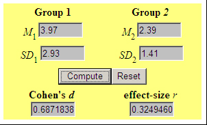
Note that the Cohen's d rounds to .69 which is considered a large effect size. The relationship would be written as follows in the body of the paper:

t (48) = 2.36, p = .01 (one-tailed), d = .69

The relationship between gender and viewing frequency could therefore be called "highly significant" and "large" when discussing the findings.

Note that Cohen's d is NOT an accurate measure of magnitude when applied to a t test for related means.

There are a variety of statistics associated with each measure of significance which are coming to be accepted as appropriate corresponding measures of effect size (magnitude). At present Cohen's d has the most widely accepted scale for interpreting the results. It is also popular because the independent t test is so widely used in many types of research.

---

While not as accepted as Cohen's d, there is a similar statistic known as eta squared (η²) which is used to measure effect size with ANOVA, which is used to measure significance when your independent variable has more than 2 values.

There are reasonably well accepted values for interpreting η². They are:

.01 - .05      Small Effect Size
.06 - .13      Medium Effect Size
    > .13      Large Effect Size

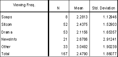
In the table below is displayed the descriptive values of data comparing viewing frequency with type of program.

Some versions of SPSS calculate eta squared (η²) for you, but it can be computed using a simple calculator to perform the following equation:

η² = Between Groups Sum of Squares/Total Sum of Squares

The SPSS printout for the ANOVA (F test) described above is shown in the following table:

Using the formula above, η² = .03. The relationship would be written as follows (if at all) in the body of the paper:

F (4, 162) = 1.38, p = .24, η² = .03

So in your results you would report that viewing frequency and program type were not found to be significantly related. In most cases you would stop there, not including any statistics. If there HAD been a significant relationship, you would have then described it as "small."

---

Effect Size When Using Nominal Data

While harder to interpret than Cohen's d, Cramer's V is considered the best statistic to measure the effect size (magnitude) when dealing with nominal data using Chi Square as your measurement for significance. SPSS will generate Cramer's V as one of the options under crosstabulation, so calculation is not an issue.

A very "crude" interpretation of V that is generally accepted is as follows:

     <.06      Negligible Relationship
.06 - .10      Weak Relationship
.11 - .15      Moderate Relationship
.15 - .25      Strong Relationship
    > .25      Very Strong Relationship

Cramer's V for the Crosstabulation example above equals .36. The relationship would be written as follows in the body of the paper:

x² (2, N = 50) = 6.60, p = .04, V=.36

The relationship between gender and viewing frequency could therefore by called "significant" and "very strongly related."

Note that while the t test yielded a higher significance level (p = .01, "highly significant"), both Cohen's d and Cramer's V indicate a high magnitude for the relationship between gender and viewing frequency.

---

Return to TVR 400 Home Page