Understanding and being able to identify levels of measurement is essential to being able to use and interpret statistics in electronic media research. The four levels are:

l. nominal: Numerical values are assigned to categories of data. This type of measurement is not quantitative at all, but necessary for computer analysis. Can be confusing. Avoid arithmetical calculations.

2. ordinal: Usually rank ordered. May be of prime importance in proprietary research, i.e. ratings.

3. interval: The intervals between levels are equal or can be assumed to be. Used in attitude research.

4. ratio: A true zero point. Rare in mass communications research.

The power of a statistical procedure is its sensitivity to weak relationships.

The strength of a relationship should not be confused with its significance. Significance only tells us if we can generalize to the population from which the sample was drawn.

Both strength and statistical significance must be considered when determining practical significance.

Variables can also be defined as discrete or continuous. We can divide a continuous scale into discrete intervals for analysis if this is more convenient or meaningful. For a bi-modal distribution (like the distance people travel to our urban church), it is possible to arrive at a mean that represents NONE of the scores. In this case, discrete categories are much more useful.

Note the popularity of the Likert scale. In attitude testing especially a positive statement is made and the subject is asked to measure his/her agreement with it on a 5 or 7 point scale. The intervals between the steps are assumed to be equal so parametric statistics may be used.

Any instrument should be tested for reliability and validity. (See text)

BASIC STATISTICS

We will look at 4 types of simple statistics in this course.

Descriptive Statistics

1. Distribution- a collection of numbers. Not very helpful.

2. f distribution- a little more organized, but still unmanageable if you have much data.

3. Histogram- more visual.

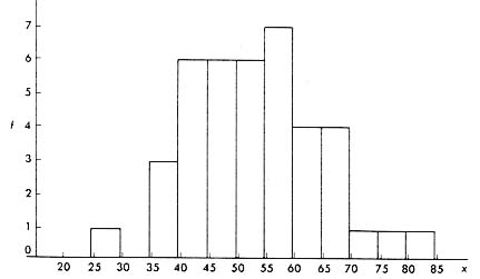
Histogram

4. f Polygon- derived from #3.


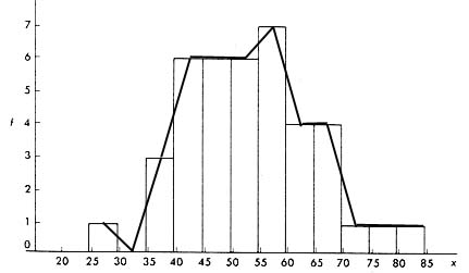
Frequency Polygon

5. Curve- we frequently smooth out the polygon.

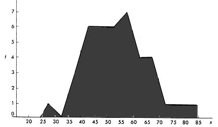
Frequency Curve

6. Normal curve- a curve which describes most behavior and other constructs as they are distributed in the total population. Most people fall in the center with progressively fewer at the extremes. Many statistical procedures are testing the fit of our obtained data with the standard distribution curve.

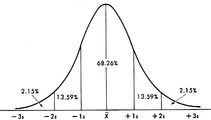
Normal Curve

Skew and Kurtosis relate to deviations from the normal curve.


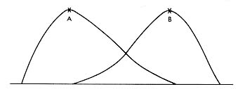
Curve A is positively skewed and Curve B is negatively skewed.

Summary Statistics

We frequently want to characterize a group of data, scores, findings, etc. by some simple number which gives the reader the general picture without having to pour over charts and tables. Several types of summary statistics include those which measure:

A. Central Tendency

Three common statistics are used:

1. mean- best for normally distributed data

2. median- minimizes influence of outlying scores

3. mode- crude and seldom of much use

B. Dispersion

These statistics describe the degree to which scores deviate from the mean.

l. range- like the mode this is crude, but it does give some insight into the nature of the distribution

2. variance- is a measure of how much the scores squared deviate from the mean squared. It is valuable, but difficult to interpret and related to the mean in each case.

3. standard deviation- is simply the square root of the variance. It is measured in the basic units of the original data.

4. standard score (z score)- it allows us to compare the variance of samples with different means in a meaningful manner. This is done by expressing raw scores in terms of SDs away from the mean.

z scores are critically important in media research because they allow for meaningful comparison of behavior data obtained using different measurements, assuming that the populations are all normally distributed.

Beware in applying parametric statistics to unknown variables that may not be normally distributed, thus negating the design of the formula.

Correlational Statistics

These statistics seek to measure the degree of association or relatedness between two variables without any assumptions of causation.

The most commonly used correlational statistic is Pearson's r which varies from -1 to +1 and thus gives a good indication of the strength of any relationship found.

Keep in mind that r by itself is just a number. It MUST be interpreted in the context of the variables being studied.

Pearson's r assumes the following:

1. both sets of scores are interval or ratio data

2. the relationship between x and y is linear and not curved

3. that both distributions are symmetrical and comparable

When any of these assumptions does not hold, use Kendall's tau or other correlation statistics which are distribution free.

Inferential Statistics

These statistics help us to judge the degree to which we can generalize the results obtained with a sample to the appropriate population.

We begin by deciding on a confidence level. This is stated in the form of the chance of our sample NOT being representative of the population and is usually set at .05 for social science research. This means that out of 100 random samples drawn from our population, we could expect the find the observed relationship between variables in 5 samples purely through the operation of chance, and without this being characteristic of the population in general.

We will be concerned primarily with 3 inferential statistics:

l. Analysis of Variance (ANOVA)- a test used for comparing the mean scores of two or more groups.

2. t-test- a special case of the ANOVA when there are only two groups (experimental and control group for example). Both ANOVA and the t-test deal with DIFFERENCES between means observed in two or more groups.

3. Chi Square (x²)- a non-parametric test making no assumptions about the distribution of the various variables in the population. This is a measure of association. Deals with FREQUENCY data only. Excellent for use with crosstabulations. Phi or Cramer's V may be used to get an idea of the strength of a relationship identified with Chi Square.

Hypothesis Testing

Once we have a well defined research problem, we can sometimes make predictions from the literature about the expected outcome of our study.

These predictions are called hypotheses and are a part of most experimental research and some empirical research.

Hypotheses provide focus to a study. They should:

1. be drawn from the literature

2. follow logical consistency

3. be stated as simply as possible

4. be testable

The null hypothesis states that any differences found between groups is the result of chance and not of any true relationship in the population.

Using the null hypothesis as a research hypothesis is dangerous as it means you will be wrong 95% of the time using standard statistical methods.

It is seldom stated.

One-tailed vs. two-tailed testing is related to whether we predict a direction to the relationship. With t-tests and ANOVA results the computer will often give both a one-tailed and a two-tailed probability. You would use the one-tailed figure if you accurately predicted the direction of the relationship and the two-tailed figure if you had no basis to predict the direction of the relationship, or if the observed relationship is opposite your prediction. While the latest APA Publication Manual allows for the identification of which type of probability you are using, in NO case would you ever report both probability figures in your results section!

Errors

Type I- rejecting the null hypothesis when it is valid

Type II- accepting the null hypothesis when it is invalid

Note that no one but statisticians really uses these terms and most professors would have to look them up to tell you which type of error is which. The important thing is to know that you as researcher have to decide which type of error is more acceptable for a particular study.

Variables which are NOT statistically significant may be very important in analyzing a relationship.

---

Return to TVR 400 Home Page